Chapter 8 Reshaping Data
Let’s say you and a colleauge are asked to support data analysis of a school. You are asked to look at the grades of five students. For each student you need to look at the their grades in different subjects.
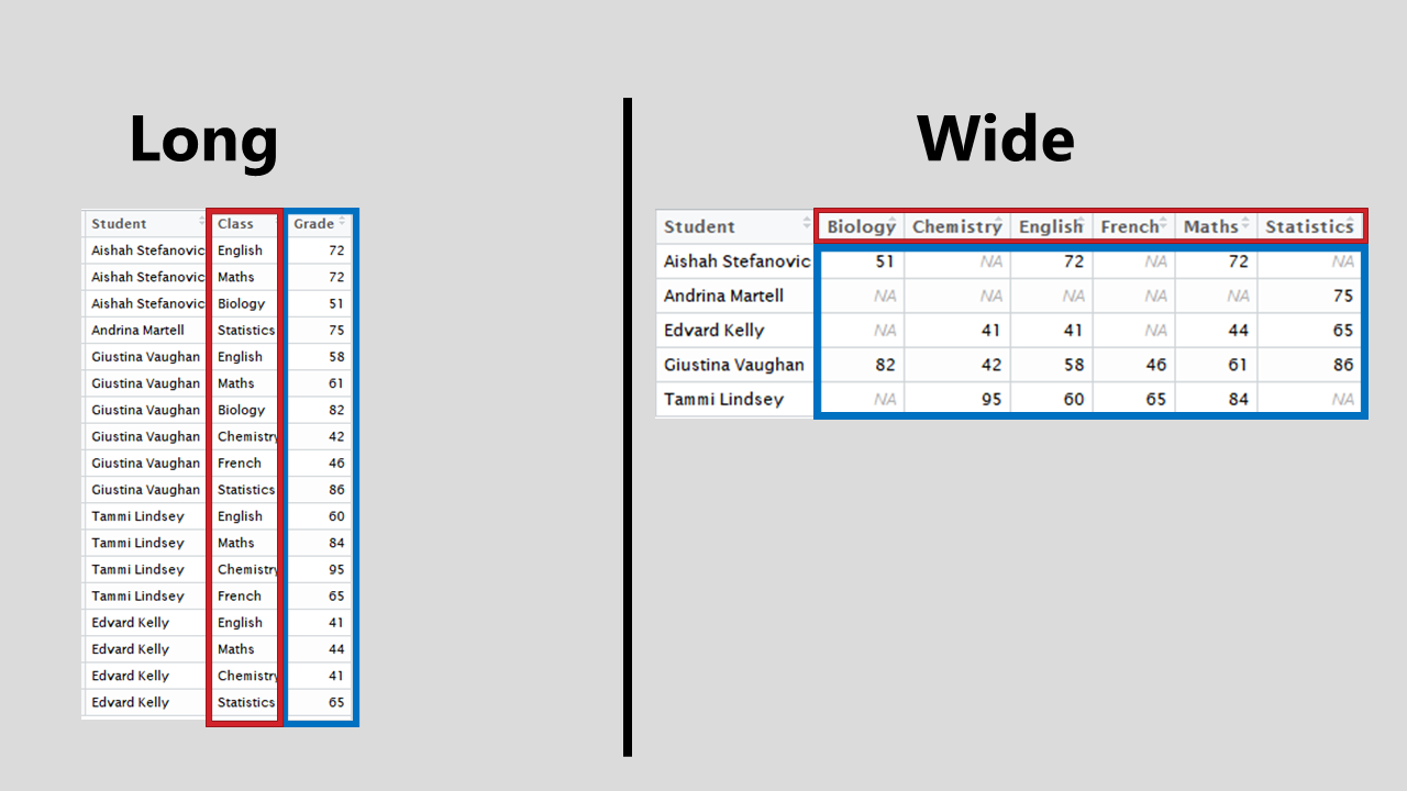
You both go away, collect your data and come back to share your results. The image below are the tables of your result. They may look different but these two datasets are showing the same information. They different only in shape; one is wide and the other is long.

Long data sets are preferrable when working on the data on a computer whereas wide formatted data works best when presenting this information. It is unlikely the problem you will be working will provide you with perfectly formatted datasets, so it is helpful to know how to move between these shapes.
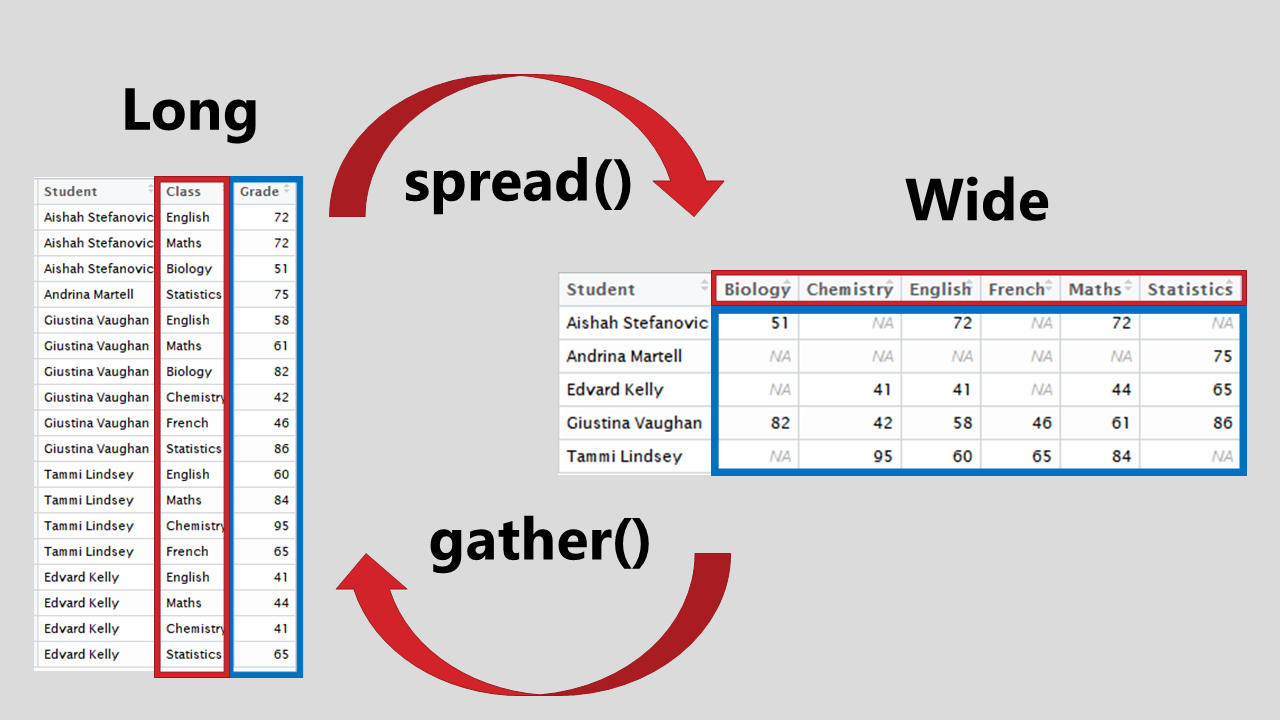
tidyr is a R package that aims to solve this problem by adding two useful “words” to our vocabulary gather() and spread().

For these functions, you need to identify two things; key and value. key is the identifier and value are the measurements. In the example, the key identifier is Class, highlighted in red and value are the Grades, highlighted in blue.
8.1 Going Long
Let’s try to apply these concepts to the the dataset we merged together in the last tutorial.
After loading the UK and Ireland data sets, run the code below to merge the datasets into one.
UKIrelandLivestock<-inner_join(UKIreland,Livestock,by=c("country"="Area","date"="Year"))## Warning: Column `country`/`Area` joining character vector and factor,
## coercing into character vectorOur task is to adjust the number of livestock in each category for the country population. This might provide a fairer comparison between the UK and Ireland over time.
QUESTION: Write a line of code to calculate a column containing the number of Turkeys per capita in the merged dataset
Currently our livestock information is in wide format: one column for each type of livestock containing the values. For our data processing it would be more efficient to work with data in long format: two columns - the first containing an identifier for livestock type and the second containing the values.
We could apply a similar function on every single livestock column in our data. This would be quite tedious! Or we could gather() our livestock columns together and then divide one single column by the population.
There are 3 arguments which are required for gather();
The first is the new name for the column which will contain the key. This will take the values that are currently assigned to the column names.
The second is the new name for the column which wil contain the values, which will contain the data values from the columns.
The third is to identify which columns to include. If these columns are sequential we can use a shortcut by using a colon and saying: FirstColumn:LastColumn
An option to use in our function is na.rm=TRUE. This will remove any missing values from our data. There are no camels as livestock in the British Isles, so adding this option will remove the rows about camels from the data
UKIrelandLivestock %>%
  gather("livestock","total",Beehives:Turkeys,na.rm=TRUE)
The same could also have been achived by fully specifying each of the columns to be gathered, and only choosing the animals relevant to the British Isles
UKIrelandLivestock %>%
  gather("livestock","total",Cattle,Chickens,Ducks,Goats,Horses,Pigs,Sheep,Turkeys)
QUESTIONS: Extend the previous line to add in a column of livestock per capita using the mutate function and assign it to a new object called UKIrelandLivestockCap
UKIrelandLivestockCap<-
  UKIrelandLivestock %>%
  gather("livestock","total",Beehives:Turkeys,na.rm=TRUE) %>%
  ?????
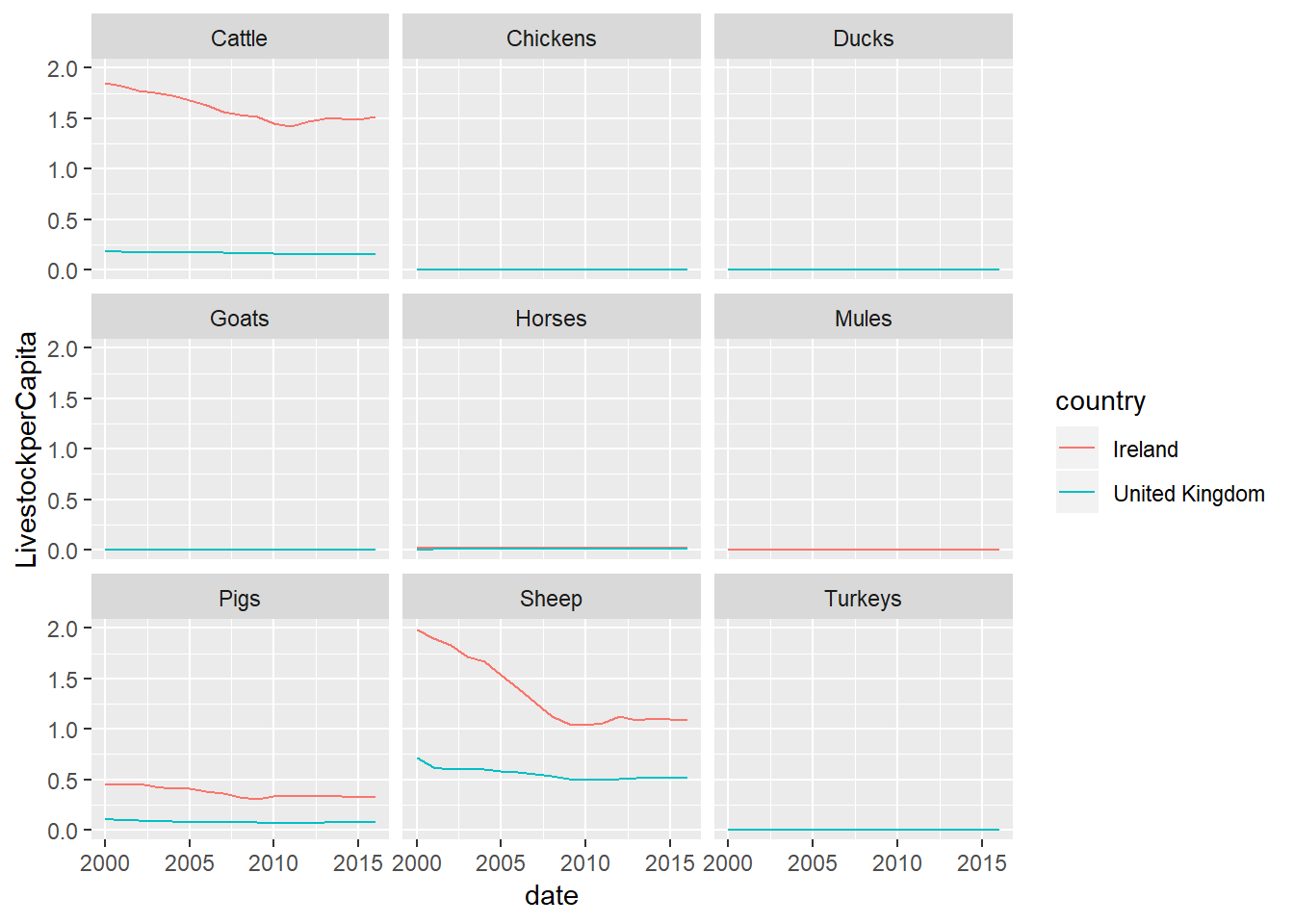
Gathering multiple columns is also a really useful way to be able to plot multiple variables in the same ggplot.
UKIrelandLivestockCap %>%
    ggplot(aes(y=LivestockperCapita,x=date,colour=country))+
        geom_line()+
          facet_wrap(~livestock)
Did this work for you? If not why not? - what needs to be changed?
This graph is a little confusing right now. Too many of the animals have very small numbers so are effectively invisible.
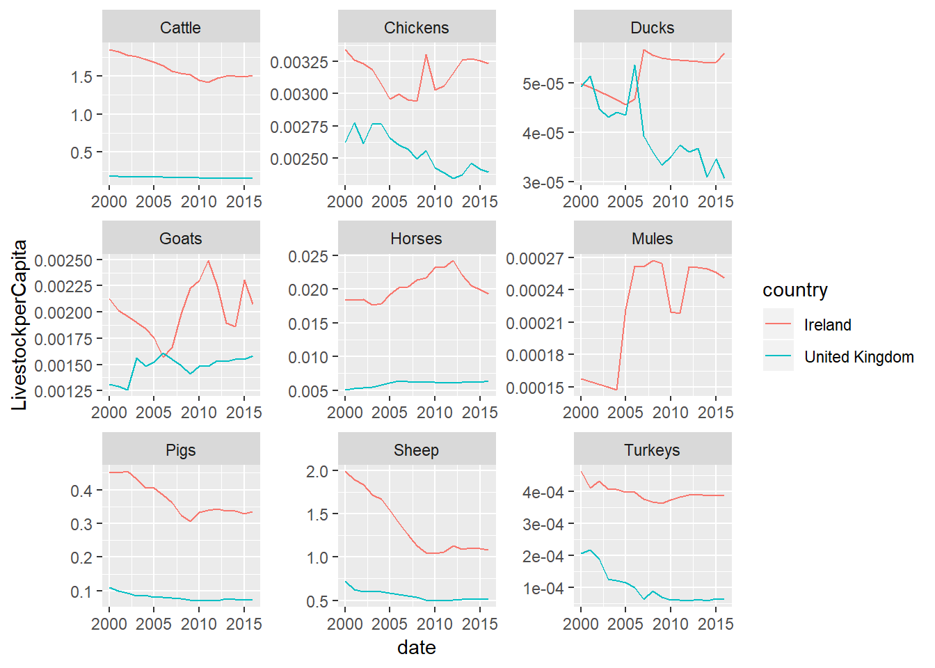
So let’s make it better - we can set our facets to have different scales using the option scales=“free”
UKIrelandLivestockCap %>%
    ggplot(aes(y=LivestockperCapita,x=date,colour=country))+
        geom_line()+
          facet_wrap(~livestock,scales="free")
One thing you probably noticed (other than the fact that the sheep population is declining at an alarming rate), is that this graph is a little bit squashed in at the moment within the RMD file. You can press the small square button in the top right corner of the plot to open a new window to view, and re-size the graph. It’s best to use a little bit of trial and error to get a graph the size you want it to be.
8.2 Going wide
When presenting results, we usually want to put the data back into a wide format as this is easier for humans to read.
Let’s say we would like to present the cattle per capita figures for UK and Ireland over the time period.
Spread requires two arguments.
The first is the column containing the identifying information. Each unique value in this column will be a column name in our wide data
The second is the column containing the corresponding values. These will form the data within each column in the wide data.
UKIrelandLivestockCap %>%
     filter(livestock=="Cattle") %>%
       select(date,country,LivestockperCapita) %>%
         spread(country,LivestockperCapita)
QUESTION: What happens if you do not include the select() line in the code? Can you explain why?
UKIrelandLivestockCap %>%
     filter(livestock=="Cattle") %>%
         spread(country,LivestockperCapita)
8.2.1 Exercises
QUESTION Read in the data frame used in the lecture notes with the information from a school database of classes, grades and students. This can be found at: http://shiny.stats4sd.org/Reading_R/Class Data.xlsx or in the data folder in RStudio Cloud
Grades<-
Classes<-
Students<-
QUESTION: Using the example from the lecture notes summarising the average grade in each class as a starting point (reproduced below): i) Produce a summary of the average grade achieved by each student; ii) The number of classes that student attended; iii) Then merge this data with the Students data frame containing the student-level information
Grades %>%
  group_by(Class) %>%
    summarise(GradeAverage=mean(Grade) ,Students=n()) %>%
        full_join(Classes,by="Class")
QUESTION: From the Livestock dataset produce a table with one column for each year showing the total number of Chickens for France
Livestock %>%
  filter() %>%
    select() %>%
      spread()
QUESTION: From the UKIreland data gather the columns gdp, population and unemployment to be able to produce a facetted plot showing all of these variables over time for the UK and Ireland
UKIreland %>%
  gather() %>%
    ggplot(aes()) +
      facet_wrap()+
        geom_XXXX()